

Welcome back to our exciting offroad adventure in the world of computer vision! Today, we're continuing our journey into conquering computer vision with code using the powerful machine learning model called 'Unet' and the robust 'resnet50' backbone. As we discussed in part 1, we're making the most of pre-trained models to enhance our exploration. We also don't have to worry about creating these models from scratch. Fortunately, the giants before us have already taken care of building these models.
In this journey, you'll witness the technical prowess of our machines as they identify objects swiftly and segment images with precision. With the skills we're about to uncover, we'll be able to differentiate our vehicles from its surroundings in images.
But, as with any expedition, understanding the underlying mechanisms is essential. Let's dive into the technical aspects that will empower you on this quest:
Image Segmentation - Dividing the Pixel Party:
Imagine a massive pixel party, where each pixel wants to join a group based on its color and style. Image segmentation is like playing the role of an ultimate party organizer, skillfully dividing pixels into different crews. Our goal? Making sure the pixels form distinct groups, representing objects or parts of objects in the image, without causing any fashion clashes! In our case, we only have 2 different parties (classes) rocking on. The background and our vehicles.
Fully Convolutional Networks (FCNs) - Offroad Trailblazers:
In our offroad adventures, FCNs are like the trailblazers - the pioneers who fearlessly venture into uncharted territories. These networks are designed to extract essential features from the pixel landscape, just as our seasoned offroaders detect critical cues on rugged trails. FCNs lead the way in identifying significant offroad elements, keeping us on the right path to success!
Skip Connections - Bridging Offroad Features:
Offroad exploration demands versatility, just like our beloved offroad vehicles. Skip connections act as the bridges connecting low-level and high-level features, combining pixel details with global context. Just like offroaders overcoming challenging obstacles with ingenious techniques, skip connections ensure that our semantic segmentation model masters the art of fusing fine-grained pixel information with overall scene understanding.
Loss Functions - Offroad Performance Metrics:
In the offroad community, we thrive on performance metrics - how well our vehicles handle obstacles and challenging terrains. Similarly, loss functions are like the performance metrics for our semantic segmentation models. They evaluate how accurately our model predicts pixel classes and guide us in improving our offroad segmentation skills. Just like offroaders aiming for the best performance, we aim for the most accurate pixel classification!
The Code
The following is what our python script will begin:
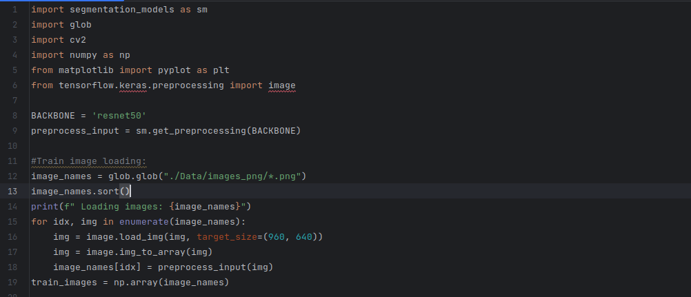
import segmentation_models as smimport globimport cv2import numpy as npfrom matplotlib import pyplot as pltfrom tensorflow.keras.preprocessing import imageThese are import statements to bring in necessary libraries and modules. Here's a breakdown:
-
segmentation_models as sm: This imports the segmentation_models library and aliases it assmfor convenience. This library provides pre-built implementations of various segmentation models. This is the library that gives us access to the pre-trained models we were nagging about. -
glob: This module is used to retrieve file names matching a specified pattern (e.g., filenames with certain extensions). -
cv2: This is the OpenCV library used for computer vision tasks. -
numpy as np: The popular NumPy library is imported and aliased asnpto work with arrays and numerical computations. -
from matplotlib import pyplot as plt: This imports thepyplotsub-module from Matplotlib, which is used for plotting data. -
from tensorflow.keras.preprocessing import image: The Keras module for preprocessing images is imported.
BACKBONE = 'resnet50'
preprocess_input = sm.get_preprocessing(BACKBONE)
-
BACKBONE = 'resnet50': This sets the variableBACKBONEto the string'resnet50'. It will be used to specify the backbone architecture for the U-Net model. -
preprocess_input = sm.get_preprocessing(BACKBONE): This retrieves the preprocessing function for the ResNet-50 backbone from thesegmentation_modelslibrary. Thepreprocess_inputfunction is used later to preprocess the images before feeding them into the model.
# Train image loading:
image_names = glob.glob("./Data/images_png/*.png")
image_names.sort()print(f" Loading images: {image_names}")
-
glob.glob("./Data/images_png/*.png"): This line usesglob.globto get a list of filenames matching the pattern"./Data/images_png/*.png". It means all PNG files in the./Data/images_png/directory. -
image_names.sort(): Theimage_nameslist is sorted alphabetically. This is to ensure the images and masks are loaded and processed in the same order. -
print(f" Loading images: {image_names}"): This line prints the list of image filenames that were loaded.
for idx, img in enumerate(image_names): img = image.load_img(img, target_size=(960, 640)) img = image.img_to_array(img) image_names[idx] = preprocess_input(img)train_images = np.array(image_names)
- This block of code loads, preprocesses, and stores the training images into the
train_imagesvariable. - The
forloop iterates through each image filename and its corresponding index usingenumerate. -
image.load_img(img, target_size=(960, 640)): This loads the image using Keras'load_imgfunction and resizes it to the target size of (960, 640) pixels. -
image.img_to_array(img): Converts the loaded image into a NumPy array. -
preprocess_input(img): Preprocesses the image using the previously obtainedpreprocess_inputfunction for the ResNet-50 backbone. - The preprocessed image is stored back into the
image_nameslist. - Finally,
train_imagesis created as a NumPy array containing all the preprocessed training images.

# Mask images loading
mask_names = glob.glob("./Data/masks/*.png")mask_names.sort()print(f" Loading masks: {mask_names}")mask_dataset = []for idx, mask in enumerate(mask_names): mask = cv2.imread(mask, 0) mask = cv2.resize((640,960)) mask = mask_dataset.append(mask/255)train_masks = np.array(mask_dataset)
- This block of code loads, preprocesses, and stores the training masks into the
train_masksvariable. - Similar to the image loading process, it uses
globto get a list of filenames matching the pattern"./Data/masks/*.png". - The masks are read using OpenCV's
cv2.imread(mask, 0), which loads the images as grayscale. - The masks are resized to (640, 960) using
cv2.resize(mask, (640, 960)). - The processed masks are stored in the
mask_datasetlist. - Finally,
train_masksis created as a NumPy array containing all the processed training masks.

python# Train val split:
train_masks = np.expand_dims(train_masks, axis=3) # May not be necessary.. leftover from previous code
from sklearn.model_selection import train_test_splitx_train, x_val, y_train, y_val = train_test_split(train_images, train_masks, test_size=0.1, random_state=42)
-
np.expand_dims(train_masks, axis=3): This line expands the dimensions of thetrain_masksarray along the third axis (axis=3) to create a single-channel mask (necessary for model training). This step is performed because the U-Net model requires input masks to have a channel dimension, even if there's only one channel (gray-scale). -
from sklearn.model_selection import train_test_split: The script imports thetrain_test_splitfunction from scikit-learn, which is used to split the dataset into training and validation sets. -
x_train, x_val, y_train, y_val = train_test_split(train_images, train_masks, test_size=0.1, random_state=42): This line splits the preprocessed images (train_images) and masks (train_masks) into training and validation sets. Thetest_size=0.1specifies that 10% of the data will be used for validation, andrandom_state=42ensures reproducibility.
# preprocess input
x_train = preprocess_input(x_train)x_val = preprocess_input(x_val)
- These lines preprocess the input data (images) using the
preprocess_inputfunction for ResNet-50, which was previously defined.
# define model
model = sm.Unet(BACKBONE, encoder_weights='imagenet',encoder_freeze=True) model.compile(optimizer='adam', loss=sm.losses.bce_jaccard_loss,metrics=[["accuracy"],[sm.metrics.iou_score]])
- The script creates a U-Net model using
sm.Unetfrom thesegmentation_modelslibrary. The model is initialized with the ResNet-50 backbone, and its encoder is initialized with weights pre-trained on the ImageNet dataset (specified byencoder_weights='imagenet'). -
encoder_freeze=Truefreezes the encoder's weights during training, meaning the pre-trained weights will not be updated. - The model is compiled using the Adam optimizer (
optimizer='adam') and the combination of binary cross-entropy and Jaccard loss (sm.losses.bce_jaccard_loss) as the loss function. - Two metrics are used for evaluation: accuracy and Intersection over Union (IoU) score.
print(model.summary())
- This line prints a summary of the model architecture, showing the number of parameters and the structure of the neural network.

history = model.fit(x_train, y_train, batch_size=1, epochs=25, verbose=1, validation_data=(x_val, y_val))
- The model is trained using the
fitmethod on the training data (x_trainandy_train). -
batch_size=1means that the model will be updated after processing each individual sample (batch size of 1). - The training is performed for 25 epochs (
epochs=25). - The training progress is displayed as each epoch is completed (
verbose=1). - The validation data (
x_valandy_val) are used for validation during training.
loss = history.history['loss']val_loss = history.history['val_loss']epochs = range(1, len(loss) + 1)plt.plot(epochs, loss, 'y', label='Training loss')
plt.plot(epochs, val_loss, 'r', label='Validation loss')
plt.title('Training and validation loss')
plt.xlabel('Epochs')
plt.ylabel('Loss')
plt.legend()
plt.show()
- These lines plot the training and validation loss over each epoch using Matplotlib. The loss values are obtained from the
historyobject obtained during training.
acc = history.history["accuracy"]val_acc = history.history["val_accuracy"]plt.plot(epochs, acc, 'y', label="Training acc")
plt.plot(epochs, val_acc, 'r', label="Validation acc")
plt.title("Training and Validation Accuracy")
plt.xlabel("Epochs")
plt.ylabel("Accuracy")
plt.legend()
plt.show()
- These lines plot the training and validation accuracy over each epoch using Matplotlib. The accuracy values are also obtained from the
historyobject.
model.save("./resnet50_unet_25epochs.h5")
- The trained model is saved to a file named
"./resnet50_unet_25epochs.h5"using thesavemethod of the model. This saved model can be loaded and reused later for predictions or further training.
And thus, dear offroading adventurers, we reach the thrilling conclusion of this captivating tutorial on the magical art of computer vision! Armed with the knowledge of preprocessing, the prowess of U-Net, and the might of ResNet-50, you are now the masters of image segmentation and object recognition in the offroad wilderness!
But hold on tight, for the most exciting chapter awaits! In Part 3 of our grand quest, we shall embark on the ultimate offroad challenge - implementing our newly trained computer vision model! Get ready for a spectacle like no other as we unleash the full potential of this enchanted creation in the real-world terrains! 💻🚙
Until then, keep honing your coding skills, for the wonders of AI are boundless in the realm of offroading! May your Python prowess continue to amaze, and may your offroad journeys be ever-thrilling! Stay curious, stay adventurous, and be ready to conquer new frontiers with our trained computer vision model in the thrilling Part 3!